Sampling from the Singular Normal
Following up the previous post on sampling from the multivariate normal, I decided to describe in more detail the situation where the covariance matrix or precision matrix is singular (e.g., it is not positive definite). A normal distribution with such a singular covariance/precision matrix is referred to as a singular normal distribution. Here is 100 samples from a two dimensional example:
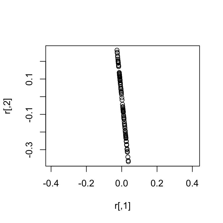 Notice that a singular normal essentially has less dimensions (in this case 1 dimension) than the dimension of the random variable (in this case 2 dimensions).
When working with singular normals lots of problems can arise, the most common is issues relating to sampling from these distributions. In these situations the Cholesky decomposition of the covariance / precision matrix will fail. If you are using R you may end up with an error like the following:
# Create singular covariance matrix
(Sigma <- crossprod(matrix(rnorm(3),1,3)))
## [,1] [,2] [,3]
## [1,] 1.932865 1.2123852 -1.5026330
## [2,] 1.212385 0.7604659 -0.9425232
## [3,] -1.502633 -0.9425232 1.1681654# This should cause an error - use safely (from purrr) so that site still renders
safely(chol)(Sigma)## $result
## NULL
##
## $error
## <simpleError in chol.default(...): the leading minor of order 2 is not positive definite>In fact even inverting this covariance matrix will run into issues as the inverse is not well defined.
safely(solve)(Sigma)## $result
## NULL
##
## $error
## <simpleError in solve.default(...): system is computationally singular: reciprocal condition number = 6.86973e-18>One solution to this problem is given by the Eigen decomposition which will not only allow us to sample from such a singular covariance matrix but it will also allow us to detect when a covariance matrix is singular.
A Key Point: The Cholesky decomposition is typically much faster than the Eigen decomposition. Therefore, if you know your covariance / precision matrix is not singular the Cholesky decomposition is typically a better choice. I described the use of the Cholesky distribution for this purpose in detailed here.
Background: The Eigen Decomposition
Any square matrix with real elements \(\Sigma\)1 can be decomposed as \[\Sigma = V_\Sigma D_\Sigma V_\Sigma^T\] where \(V\) is a matrix of orthonormal column vectors (called the Eigenvectors) and \(D\) is a diagonal matrix with diagonal elements called Eigenvalues that are decreasing (that is \(D_{ii} \geq D_{(i+1)(i+1)}\)).
Lots of great stuff has been written about the Eigen decomposition, rather than rehash these topics here I will instead just point out that the Eigen decomposition can be used to find a matrix square root (just like the Cholesky). Remember that the square root of a matrix \(\Sigma\) is defined by the relation \(\Sigma = \Sigma^{\frac{1}{2}}\left(\Sigma^{\frac{1}{2}}\right)^T\). For the Eigen decomposition we can write \[\Sigma = V_\Sigma D_\Sigma^{\frac{1}{2}}\left(V_\Sigma D_\Sigma^{\frac{1}{2}}\right)^T\] where \(D^{\frac{1}{2}}\) is essentially the same and \(D\) but where the diagonal is given by the square root of the Eigenvalues (rather than by the Eigenvalues). This shows that \(VD^{\frac{1}{2}}\) is a matrix square root and suggests we can use this in place of the Cholesky factor in sampling from the multivariate normal.
The Eigen decomposition is also rank revealing (it will tell you if your covariance/precision matrix is singular and if so how singular it is). Cutting to the chase, a symmetric positive definite matrix \(X\) is a symmetric matrix where all the Eigenvalues are positive. If all the Eigenvalues are negative its symmetric negative-definite. If a \(p\times p\) symmetric matrix \(X\) has \(k < p\) positive Eigenvalues and \(p-k\) zero Eigenvalues then we say \(X\) is symmetric positive semi-definite (e.g., singular and of rank \(k\)). If some Eigenvalues are positive and some are negative and you expected \(X\) to be a covariance / precision matrix… something has gone very wrong2.
So lets take a look at the Eigen decomposition of the matrix Sigma that was giving us trouble above.
(es <- eigen(Sigma))## eigen() decomposition
## $values
## [1] 3.861496e+00 2.220446e-15 0.000000e+00
##
## $vectors
## [,1] [,2] [,3]
## [1,] -0.7074943 0.7067191 0.0000000
## [2,] -0.4437742 -0.4442610 0.7782651
## [3,] 0.5500148 0.5506181 0.6279358Note that only one of the Eigenvalues is positive and the other two are zero3; this means that Sigma is positive-semidefinite (singular of rank 1).
Sampling from the Singular Normal
Just as I introduced regarding sampling from the non-singular multivariate normal, here we are going to use the non-centered parameterization to generate singular normal random variables from univariate standard normal (mean zero variance 1) draws. To sample \(n\) draws form a \(p\) dimensional singular normal distribution let us introduce the \(p \times n\) matrix \(Z\) with elements \(Z_{ij} \sim N(0, 1)\).
Covariance Parameterization
To sample \(X \sim N(\mu, \Sigma)\) where \(\Sigma\) is a \(p\times p\) potentially singular covariance matrix, we have the following non-centered relationship \[X = \mu + V_\Sigma D^{\frac{1}{2}}_\Sigma Z\]
Note that if \(\Sigma\) is of rank \(k< p\), there is some redundancy here: \(Z\) can actually be of dimension \(k \times n\) and we can simply take the first \(k\) columns of \(V_\Sigma\) and \(D^{\frac{1}{2}}_\Sigma\) and we will still get the same answer.
Precision Parameterization
To sample \(X \sim N(\mu, \Omega)\) where \(\Omega\) is a \(p\times p\) potentially singular precision matrix, we have the following non-centered relationship \[X = \mu + V_\Omega D^{-\frac{1}{2}}_\Omega Z\] Here the only difference compared to the covariance parameterization is that the elements of \(D^{-\frac{1}{2}}_\Omega\) are given by \(1/\sqrt{D_{ii}}\).
Again, note that if \(\Omega\) is of rank \(k< p\), there is some redundancy here: \(Z\) can actually be of dimension \(k \times n\) and we can simply take the first \(k\) columns of \(V_\Omega\) and \(D^{\frac{1}{2}}_\Omega\) and we will still get the same answer.
Code
Below I demonstrate code designed to sample from the singular multivariate normal in either parameterization. In particular, note that these functions make use of the truncation I mentioned above that reduces the redundancy in the non-centered distribution for the singular normal case.
Also notice that these functions can be used to sample from non-singular multivariate normal distributions as well. In this way these functions are more general than those given previously but they are typically slower because they use the Eigen decomposition rather than the Cholesky.
#' Truncated Eigen Square Root (or inverse square root)
#'
#' Designed for Covaraice or Precision matricies - throws error if
#' there is any large negative Eigenvalues.
#'
#' @param Sigma p x p matrix to compute truncated matrix square root
#' @param inv (boolean) whether to compute inverse of square root
#' @return p x k matrix (where k is rank of Sigma)
trunc_eigen_sqrt <- function(Sigma, inv){
  es <- eigen(Sigma)

  # Small negative eigenvalues can occur just due to numerical error and should
  # be set back to zero.
  es$values[(es$values < 1e-12) & (es$values > -1e-12)] <- 0

  # If any eigen values are large negative throw error (something wrong)
  if (any(es$values < -1e-12)) stop("Non-trivial negative eigenvalues present")

  # calculate square root and reveal rank (k)
  k <- sum(es$values > 0)
  if (!inv){
    L <- es$vectors %*% diag(sqrt(es$values))
  } else if (inv) {
     L <- es$vectors %*% diag(1/sqrt(es$values))
  }
  return(L[,1:k, drop=F])
}

#' Covariance parameterization (Eigen decomposition)
#' @param n number of samples to draw
#' @param mu p-vector mean
#' @param Sigma covariance matrix (p x p)
#' @return matrix of dimension p x n of samples
rMVNormC_eigen <- function(n, mu, Sigma){
  p <- length(mu)
  L <- trunc_eigen_sqrt(Sigma, inv=FALSE)
  k <- ncol(L)
  Z <- matrix(rnorm(k*n), k, n)
  X <- L%*%Z
  X <- sweep(X, 1, mu, FUN=`+`)
}

#' Precision parameterization (Eigen decomposition)
#' @param n number of samples to draw
#' @param mu p-vector mean
#' @param Sigma precision matrix (p x p)
#' @return matrix of dimension p x n of samples
rMVNormP_eigen <- function(n, mu, Sigma){
  p <- length(mu)
  L <- trunc_eigen_sqrt(Sigma, inv=TRUE) # only difference vs. cov parameterization
  k <- ncol(L)
  Z <- matrix(rnorm(k*n), k, n)
  X <- L%*%Z
  X <- sweep(X, 1, mu, FUN=`+`)
}
Now we just check that the mean and covariance of each function matches what it should be (using the same Sigma we defined above).
n <- 10000
mu <- 1:3
Omega <- MASS::ginv(Sigma) # use pseudoinverse
x1 <- rMVNormC_eigen(n, mu, Sigma)
x2 <- rMVNormP_eigen(n, mu, Omega)

# Create function that tests for equality with high tolerance due to
# random number generation
weak_equal <- function(x, y) all.equal(x, y, tolerance=.05)

# check row means match up with mu and agree with eachother
weak_equal(rowMeans(x1), mu) & weak_equal(rowMeans(x2), mu)
## [1] TRUE# check empirical covariances agree
weak_equal(var(t(x1)), var(t(x2)))## [1] TRUENote that we used the pseudo-inverse of Sigma above to create a rank-deficient precision matrix (Omega) that should correspond to the same distribution as Sigma.
Note this is more general than for just symmetric positive definite matrices as in the definition of the Cholesky decomposition introduced previously↩
I only really see this when using Laplace approximations and when the optimization ended at a saddle point rather than at the Maximum a Posteriori estimate.↩
any slight non-zero number in either of the last two Eigenvalues is just due to numerical errors in the calculation of the Eigen decomposition↩