Framing the decision space

I first need to introduce some formal way in which we discuss “decisions”. For a given problem, imagine that there is a space in which all of my possible decisions live. This space can be discrete, continuous, multivariate, or any number of crazy things based on the problem at hand. In what follows I will denote our decision space (regardless of what exactly it is) by \(\mathcal{A}\) and a decision \(a\in \mathcal{A}\).

The other information that helps us make a decision

In Bayesian decision theory we are concerned with choosing between these different decision based on some information. Like our decision space, there is tremendous flexibility in what our information is (univariate, multivariate, continuous, discrete, etc…). Whatever that information is I will denote the space that our information lives in by \(\Theta\) and a piece of information (one element of this space) by \(\theta\) such that \(\theta \in \Theta\).

The Loss Function

So how do we determine the “best” decision? This requires that we first define some notion of what we want (what are we trying to do?). The formal object that we use to do this goes by many names depending on the field: I will refer to it as a Loss function (\(\mathcal{L}\)) but the same general concept may be alternatively called a cost function, a utility function, an acquisition function, or any number of different things. The crucial idea is that this is a function that allows us to quantify how bad/good a given decision (\(a\)) is given some information (\(\theta\)).

What does it mean to quantify? By convention I mean a real number (between \(-\infty\) and \(+\infty\)). Here I will be discussing “Loss functions” and this real value will reflect the loss we feel if we choose decision \(a\) given our information \(\theta\). We may denote this loss function as

\[\mathcal{L}: \Theta\times\mathcal{A} \rightarrow \mathcal{R}\]

The crucial idea is that the loss function ties together our decision space (\(\mathcal{A}\)) and our information space (\(\Theta\)).

I find that the hard part of decision theory is often the choice of the loss function; this is really a subjective choice that should capture what matters to you. In the following examples I will focus on just a few very simple examples.

Uncertainty

I have written before on how crucial it can be to quantify our uncertainty in analyses or estimates. In short, it is one thing to estimate a quantity, but it can be far more powerful to not only estimate a quantity but actually quantify our uncertainty about an estimate as a distribution over possible values.

Rather than just dealing with a single known value for \(\theta\in \Theta\) we now work with a probability distribution representing our belief in the “true” value of \(\theta\) which I will denote by \(p(\theta)\). To connect this to Bayesian statistics, we may have a posterior distribution over \(\theta\) conditioned on some observed data \(x\). It is because Bayesian statistics is often about calculating these posterior distributions that most Bayesian texts on decision theory discuss this uncertainty of information as \(p(\theta|x)\). However, any probability distribution over our information space can be used here. For example, we could obtain a distribution over \(\theta\) through error propagation of another measured or guessed quantity as I discussed in a previous post.

So how do we figure out the loss associated with individual decisions when we don’t even know the information we want to use to make a decision? The answer is that we turn to probability theory and instead calculate the “Expected Loss” we would feel if we choose a given action given our beliefs (our probability distribution) about \(\theta\). We calculate this “Expected” loss just like we would calculate the expectation of any other function of a random variable.

\[\text{Expected Loss}(a) = \int_\Theta\mathcal{L}(\theta, a)p(\theta)d\theta\] Essentially the expected loss sums up the loss we would feel for a given decision \(a\) over all possible values of our information \(\theta\) but weighted by the probability of \(\theta\). So why should we care about this? In this form the Expected Loss does some pretty remarkable things in terms of decision making. In particular, the Expected Loss balances between how probable each value of \(\theta\) is and the loss associated with each value of \(\theta\) for a given \(a\).

In what follows, we will not calculate this integral directly but instead use \(N\) samples \((\theta^{(1)}, \dots, \theta^{(N)})\) from the distribution \(p(\theta)\) to approximate this integral by

\[\text{Expected Loss}(a) \approx \frac{1}{N}\sum_{n=1}^N\mathcal{L}(\theta^{(n)}, a).\] This is what I meant at the start of this post when I said we would rely on simulation rather than analytical closed form solutions (more on this at the end of the post).

Finally we come to the hard part. We need to pick a given value of \(a\) that is “best”. By best we will mean the decision that has the lowest expected loss. Will call the decision that minimizes the Expected Loss the “Bayes Action” and denote it \(\hat{a}\) such that

\[\hat{a} \approx \underset{a\in \mathcal{A}}{\text{argmin}} \frac{1}{N}\sum_{n=1}^N\mathcal{L}(\theta^{(n)}, a). \] Why did I say this was the hard part? Because this part can get computationally intense quickly. Even if we were not using simulations and instead solving this optimization explicitly, analytical closed form solutions are only possible for a select set of loss functions and distributions \(p(\theta)\) (more on this at the end of the post).

Here, rather than continuing to go through the examples in the same manner I have done so far, I will instead focus just on the first example and go start-to-finish through a full worked Bayesian decision theory problem.

Fully Worked Example: What price should I sell my used phone for?

Imagine I have an unscratched used phone that was made in 2014 that I want to sell. I might go online and look at some closed eBay listings and see what sold and what didn’t. Lets pretend I believe that there are 3 key variables that dictate whether a phone sold or not: whether it was scratched or not, the year it was made, and the price it was listed at. Given this information I want to figure out what price I should list my phone at. In particular I want to maximize my expected return (the expected amount of money I will make), this defines my loss function as I will discuss below.

Here is some pretend data (from 6 closed eBay listings) from such an exercise where I have denoted whether a phone sold with a 1 and if it didn’t with a 0 (same for whether or not it was scratched).

library(tidyverse)
library(brms)

d <- data.frame(sold = c(1, 1, 0, 0, 1, 1), 
           scratched = c(0, 0, 1, 0, 0, 0), 
           year = c(2014, 2015, 2010, 2014, 2015, 2016), 
           price = c(50, 70, 40, 100, 90, 100))
d

##   sold scratched year price
## 1    1         0 2014    50
## 2    1         0 2015    70
## 3    0         1 2010    40
## 4    0         0 2014   100
## 5    1         0 2015    90
## 6    1         0 2016   100

Lets fit a very simple Bayesian Logistic Regression model to this data. Here is the model:

\[\begin{align} y_{\text{sold}, i} &\sim \text{Bernoulli}(\pi_i) \\ \pi_i &= \text{Logit}^{-1}(\eta_i) \\ \eta_i &= \beta_0 + \beta_\text{1}x_{\text{scratched},i} + \beta_\text{2}x_{\text{year},i} + \beta_\text{3}x_{\text{price},i} \end{align}\]

We will use a default uniform prior on \(\beta_0\) and we will place informative priors on the other coefficients. For example, since I believe that having a scratch would likely decrease the probability that a phone sold I will use the following prior \(\beta_1 \sim \text{Normal}(-1, 1)\).

fit <- brm(sold ~ scratched + year + price, data = d, family = bernoulli(link = "logit"), 
           prior = c(set_prior("normal(-1,1)", class="b", coef="scratched"), 
                     set_prior("normal(1, 1)", class="b", coef="year"), 
                     set_prior("normal(-2, 1)", class="b", coef="price")), 
           silent=TRUE, 
           refresh = -1)

## 
## Gradient evaluation took 3.9e-05 seconds
## 1000 transitions using 10 leapfrog steps per transition would take 0.39 seconds.
## Adjust your expectations accordingly!
## 
## 
## 
##  Elapsed Time: 0.056959 seconds (Warm-up)
##                0.035268 seconds (Sampling)
##                0.092227 seconds (Total)
## 
## 
## Gradient evaluation took 6e-06 seconds
## 1000 transitions using 10 leapfrog steps per transition would take 0.06 seconds.
## Adjust your expectations accordingly!
## 
## 
## 
##  Elapsed Time: 0.059337 seconds (Warm-up)
##                0.02873 seconds (Sampling)
##                0.088067 seconds (Total)
## 
## 
## Gradient evaluation took 6e-06 seconds
## 1000 transitions using 10 leapfrog steps per transition would take 0.06 seconds.
## Adjust your expectations accordingly!
## 
## 
## 
##  Elapsed Time: 0.060765 seconds (Warm-up)
##                0.033488 seconds (Sampling)
##                0.094253 seconds (Total)
## 
## 
## Gradient evaluation took 6e-06 seconds
## 1000 transitions using 10 leapfrog steps per transition would take 0.06 seconds.
## Adjust your expectations accordingly!
## 
## 
## 
##  Elapsed Time: 0.056948 seconds (Warm-up)
##                0.03405 seconds (Sampling)
##                0.090998 seconds (Total)

summary(fit)

##  Family: bernoulli(logit) 
## Formula: sold ~ scratched + year + price 
##    Data: d (Number of observations: 6) 
## Samples: 4 chains, each with iter = 2000; warmup = 1000; thin = 1; 
##          total post-warmup samples = 4000
##     ICs: LOO = NA; WAIC = NA; R2 = NA
##  
## Population-Level Effects: 
##           Estimate Est.Error l-95% CI u-95% CI Eff.Sample Rhat
## Intercept -4310.14   1620.15 -7609.58 -1334.14       2505 1.00
## scratched    -1.16      1.00    -3.13     0.81       3185 1.00
## year          2.15      0.81     0.67     3.79       2500 1.00
## price        -0.12      0.08    -0.30     0.03       2196 1.00
## 
## Samples were drawn using sampling(NUTS). For each parameter, Eff.Sample 
## is a crude measure of effective sample size, and Rhat is the potential 
## scale reduction factor on split chains (at convergence, Rhat = 1).

Now that we have our fitted model based on our data (that is, now that we have \(p(\theta|x)\)) we can build our loss function and use our fitted model to figure out the optimal price to list my phone at.

As I said, the “loss” function I will choose is based on maximizing my expected return. Note that in this case I say “Loss function” but in reality its a function that measures the expected return and we want to maximize it. Its really just a convention as I have been calling the thing the loss function throughout this post and so I will continue to do so. However, now we want to maximize this function. This defines probably one of the simplest loss functions I could choose in this setting:

\[\mathcal{L}(\pi^*(\text{price}), \text{price}) = \pi^*(\text{price})\times\text{price}.\] Notice that I made this loss function in terms of \(\pi^*(\text{price})\) which I use to denote the probability that my phone will sell if I list it as that particular price. Just like one of our previous examples, in this case our information is actually a function of our action! It is a function that takes in the price and outputs a value between 0 and 1 (a probability). While this may seem weird and bewildering, notice that we can simply use our fitted model to predict \(\pi^*(\text{price})\).

I will implement this expected loss calculation as an R function next.

loss <- function(price){
  # First Create the input data to predict with out model - we want to predict whether or not our phone will sell
  our.phone <- data.frame(scratched=0, year=2014, price=price) 
  
  # Next, for each posterior sample from out model, predict whether or not our phone would sell at the given price. This will give a vector of 0's and 1's, did the phone sell in each posterior sample. Think of each posterior sample as a simulation. 
  pp <- posterior_predict(fit, newdata=our.phone)
  
  # Next calculate the expected return for each of these posterior simulations
  mean(pp*price)
}

Now that we have a function implementing the calculation of expected loss for each price we can optimize this to find the listing price that maximizes our expected return. Again because our “loss” function is something that in this case we want to maximize I will instead pass it to R’s optim function as a negated version of itself (add a negative sign) as the optim function defaults to minimizing a passed function.

(op <- optim(50, function(x) -loss(x)))

## $par
## [1] 71.71875
## 
## $value
## [1] -58.41492
## 
## $counts
## function gradient 
##      177       NA 
## 
## $convergence
## [1] 10
## 
## $message
## NULL

Therefore we find that the optimal listing price should be 72 and at this value we expect to make 58 dollars (or whatever your favorite currency is).

Finally lets look at what this expected return/loss looks like evaluated at a number of different listing prices.

x <- 10:110 # Listing prices to evaluate
l <- sapply(x, loss) 
plot(x, l, xlab = "Listing Price", ylab = "Expected Return")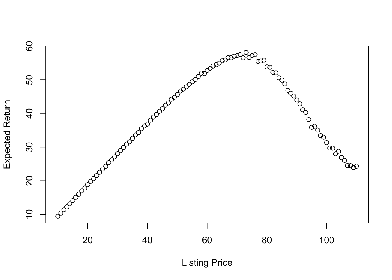

So whats the intuition behind this result? Basically if we list our phone for a low-enough value (e.g., for 10) we are almost certain that the phone will sell but we won’t make much money for it and on average we can expect to make about 10. At the other extreme if we list our phone for too much (e.g., for 110) then we are unlikely to sell it but if we do sell it, it will make much more money. Where is the best balance in terms of maximizing the expected return? Right around 71 where we can expect to make about 58 on average, just as we saw from our black-box optimization using the optim function.

Next steps

Here I have relied on simulation for both the approximation of posterior distributions \(p(\theta|x)\) and on black box optimization routines for calculating the Bayes action (\(\hat{a}\)). While I believe this approach will provide a very powerful introduction to Bayesian decision theory, readers should be aware that many optimization problems can become too computationally challenging to solve through simulation methods like this. Alternatively in some cases exact close form results are desired. Depending on the chosen loss function and on the form of the information/posterior distribution, analytical closed form solutions may be able to be found. To summarize, with some extra work, you may be able to find an explicit closed form solution for the Bayes action; doing this can pay off as it will almost certainly be more computationally efficient and can provide greater insight into the decision making process.

Many areas of engineering control theory are basically one large Bayesian decision problem where the solutions are too difficult to calculate through simulation and instead closed form calculations through either dynamic programming, calculus of variations, or other methods must be sought. In particular those interested in learning more about this should look up the Linear Quadratic Regulator (or the related Linear Quadratic Gaussian problem).

For those interested in learning more about Bayesian decision theory, my recommendation is based on how much of this post you understood. If you understood the majority of it then I would recommend thinking about this regularly and trying to use the general framework I provide in the fully worked example to preform your own analyses. Alternately, if you are like me, you may just want to go sit in a dark room and think about how many different types of loss functions you can think of. Try coming up with some involved examples that are actually functions! You don’t really need to know to much about functional analysis at this point. Alternatively, if you did not understand this post or are certain that reading more about Bayesian decision theory is necessary for you: you may want to pick up a copy of James Berger’s Book Statistical Decision Theory and Bayesian Analysis.