Error Analysis Made Ridiculously Simple
Introduction
All measurements have uncertainty. This is not a subjective opinion but an objective fact that should never be ignored. In light of this, I have always been curious about how infrequently uncertainty is actually taken into account in science.
In this post I will advocate the use of simple simulation studies for error/uncertainty propagation. For our purposes, I will use the concepts of error and uncertainty interchangably.
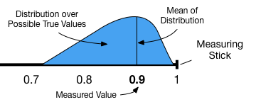
When I talk about uncertainty I am talking about a probability distribution over possible true values given our measurement. Often our distribution will be centered and symmetric about the value we measured but it need not be. A typical choice of distribution is a normal distribution with mean equal to our measured value and a standard deviation that is dictated by the precision of our measurement device.
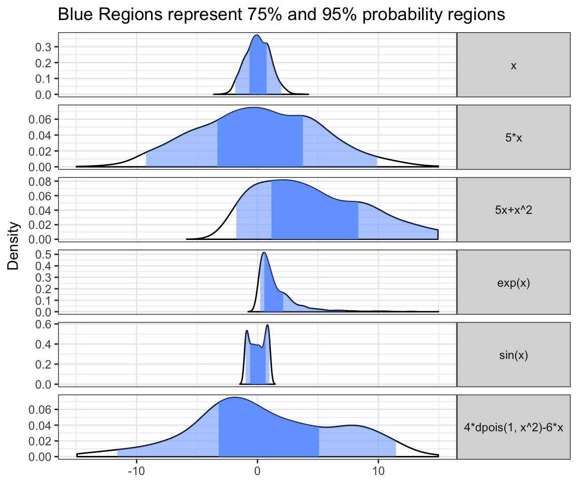
So what is propogation of uncertainty? Imagine that I measure \(x\) but am interested in calculating \(y\) where \(y = f(x)\). Since I know that there is uncertainty in my measurement of \(x\), I need to figure out the resulting uncertainty in my calculation of \(y\). This is actually a crucial concept. Imagine that \(y = x^{1000}\), it should be fairly obvious that small errors in the measurement of \(x\) can lead to massive errors in the value of \(y\). What about for arbitrary functions and arbitrary distributions of error/uncertainty? Just to give a very quick example. Imagine that I measure \(x\) such that the resulting uncertainty in the true value of \(x\) is given by \(x \sim \mathcal{N}(0,1)\). In the following figure I show the distribution of our uncertainty in \(x\) and the distribution of uncertainty in a number of calculated quantities \(y=f(x)\). Notice that the resulting distributions may not be normally distributed and are not necessarily easily intuited.
There is actually an entire field of mathematics devoted to Error Analysis. Unfortunately, this subject is often taught with a bunch of formulas that need to be learned without much emphasis on understanding the concepts or intuition. However, with the abundance of computing resources available nowadays, I would advocate simulation studies to understand and do propagation of error calculations rather than learning these formulas as a starting point. I also feel that simulation studies will provide greater generalizability than many of the techniques taught in an introductory course on error analysis.
What can you do with all this? What I am advocating is a very general idea that can be used in many different ways. Here are a few examples:
Imagine you are reading a paper where the authors claimed to have used a given method to measure a quantity \(x\) which is used to calculate a quantity of interest \(y\). Before you even see their results, you may want to estimate whether you believe that they have sufficient accuracy/precision in their measurement of \(y\) to address their hypothesis or support their claims based on the uncertainty in their measurement of \(x\).
Imagine you are designing a study and you want to estimate the sample size needed so that you can calculate a quantity of interest \(y\) with a given level of uncertainty. This is very similar to the idea of power calculations that are often done when designing experiments.
Imagine you want to “guesstimate” a value \(y\) based on your guess of a quantity \(x\). You may also want to use your estimate in your uncertainty over the quantity \(x\) to estimate your uncertainty in your “guesstimate” of \(y\).
Overview of this post:
Example 1 is intended to build some intuition regarding what propagation of uncertainty is, why it is non-trivial, and to motivate and (informally) derive one of the basic formulas used in error analysis (the formula for adding two independent measurements). If you find my presentation here confusing, don’t worry, just skip to the next section and try to come back to this later if you want.
Using Simulation Studies: This section is the meat of the post and those familiar with error analysis should just skip to this section. Here I lay out just how simple it can be to do these calculations with a computer. I also show how approaching these problems through simulation can also allow an analyst to solve some really difficult problems almost trivially simply.
Comments on “Back-of-the-Envelope” calculations. Here I briefly comment about how uncertainty propagation can lead to more informative back-of-the-envelope calculations with little extra effort (spoiler: just replace “measured quantity” with “estimated/guessed quantity” in other parts of the post).
The take home message of this post is to always remember uncertainty in your calculations of measured/approximated quantities. Doing so is very powerful and can lead to better, more informative, and more robust calculations.
Example 1 - Adding two measurements
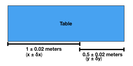
Imagine you are trying to measure the length of a long table with a meter stick but the table is longer than 1 meter. To measure the table we lay the meter stick down starting at one end, mark the end of the meter stick, then move the meter stick to the mark and measure to the end of the table as shown in the above figure. Imagine that the measurements with the meter stick have an uncertainty of \(\pm 0.02\) meters. Lets denote the first measurement by \(x \pm \delta x\) and the second by \(y \pm \delta y\). We are interested in the sum of these two measurements which we will call \(z = x+y\). Its easy to figure out \(z = x+y\), but our interest is in how to combine the uncertainties \(\delta x\) and \(\delta y\) to get the uncertainty in \(\delta z\).
The first approach is to simply add the uncertainties such that \(\delta z = \delta x + \delta y\). This approach can be useful if what you are interested in is the maximum possible uncertainty (e.g., the worst case scenario) but often this approach is overly conservative. Why do I say that this may be overly conservative? Consider that if my measurements are independent then the true value of either of our two measurements may be above or below the value we measured. If both measurements are greater than or less than their true values, then our uncertainties will add leading to a greater overall uncertainty in our combined measurement. However, if one measurement is above the true value and the other is below the true value, then some amount of the uncertainty will “cancel out”.
So what might be a more appropriate way of combining errors from independent measurements? The following formula is often taught as an alternative to simply adding the errors \[\delta z = \sqrt{(\delta x)^2+(\delta y)^2}.\]
In the next two subsections I will try to explain how we can think about these two formulas (\(\delta z = \delta x + \delta y\) vs. \(\delta z = \sqrt{(\delta x)^2+(\delta y)^2}\)) and where they come from. I am hoping that this will provide a bridge between the traditional starting point for talking about propagation of errors and my more probabilistic, simulation based, treatment.
Example 1a - Uniform Uncertainty and Max/Min Bounds
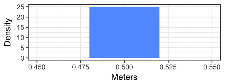
Given the setup in the above example, imagine that the uncertainty of \(\pm 0.02\) meters represents the bounds of a uniform distribution for the true value. That is, if we measured something as being 0.5 meters then the distribution of the true value is given in the following plot:
In this setup it may make sense to measure what the maximum and minimum possible bounds are on our combined measurement \(z = x+y\). This is simply given by the addition of the maximum and minimum bounds for the two measurements such that \(\delta z = \delta x + \delta y = 0.04\).
Example 1b - Gaussian Uncertainty and Standard Deviation as Bounds
What if instead we imagined that the uncertainty of \(\pm 0.02\) meters represented the standard deviation of a normal distribution centered on our measured values. Here, the distribution of our uncertainty is shown in the following graph
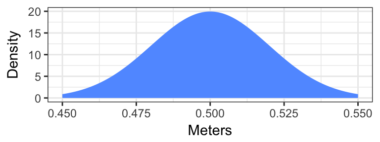
In this case, values close to our measurement are more likely than values farther away from our measurement; this is likely a more realistic situation than the uniform error example above. However, when working with a normal distribution, the maximum and minimum error don’t really make any sense. For a normal distribution, the minimum and maximum possible values are at \(-\infty\) and \(+\infty\), respectively, even though the probability of the true value being \(\pm \infty\) is actually zero. Essentially, max/min bounds are just not a useful concept if our uncertainty is distributed normally. This is one reason why we instead choose to measure the standard deviation or variance of uncertainty that is normally distributed.
Now lets do a small simulation study to determine the distribution of uncertainty in our table measurement example with normally distributed uncertainty.
iterations <- 3000 # Number of experiments to simulate
x <- rnorm(iterations, mean = 1, sd = 0.02) # simulate first measurement
y <- rnorm(iterations, mean = 0.5, sd = 0.02) # simulate second measurement
data.frame("x" = x,
"y" = y,
"z = x+y" = x+y, # simulate the addition of the two measurements
check.names=F) %>%
plot_error_quantiles() +
ggtitle("Blue Regions represent 75% and 95% probability regions") +
xlab("Meters")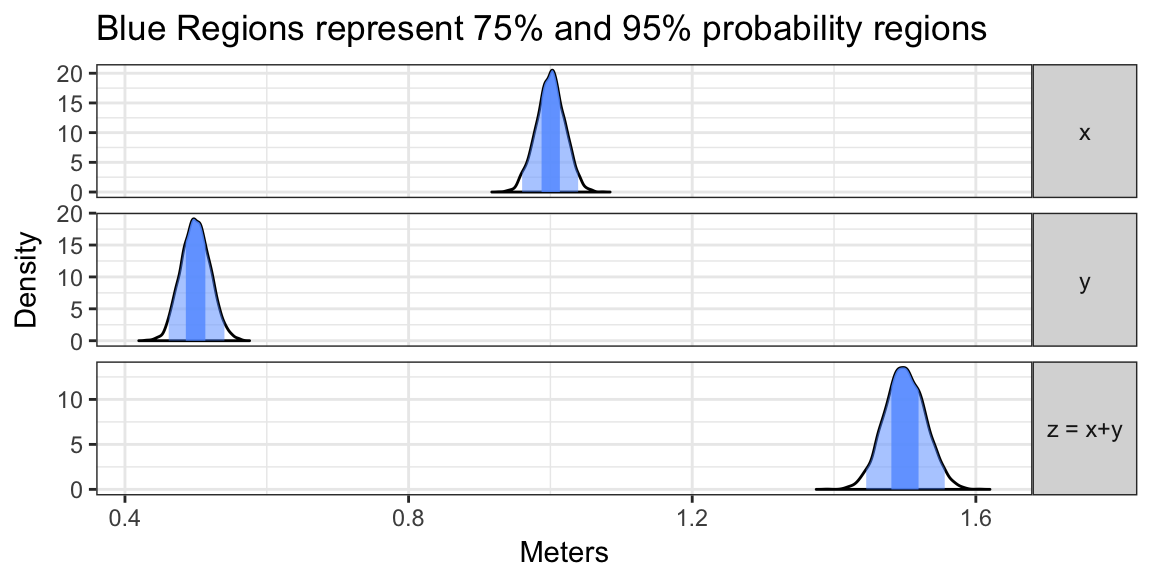 This figure shows the distribution of uncertainty in our combined measurement \(z\) given the distributions of our measurements \(x\) and \(y\). Note that the width of the distribution of \(z\) is greater than the width of the distributions for \(x\) or \(y\). But what is the standard deviation?
print(paste("Standard Deviation of Z:", signif(sd(x+y), 3)))## [1] "Standard Deviation of Z: 0.0284"print(paste("Uncertainty in Z by Square root formula:", signif(sqrt(0.02^2+0.02^2), 3)))## [1] "Uncertainty in Z by Square root formula: 0.0283"We can see that the standard deviation of \(z\) (which we have been denoting by \(\delta z\)) which we obtained from this stimulation is nearly identical to the result of that square root formula I mentioned earlier. This isn’t intended to be a proper derivation of the square root formula, instead I am just trying to point out that thinking of error as a standard deviation leads to that square root formula. A proper derivation of the square root formula (\(\delta z = \sqrt{(\delta x)^2+(\delta y)^2}\)) comes from the fact that variance of the addition of independent random variables adds (\(Var(X+Y) = Var(X)+Var(Y)\)) and \(SD(x)^2 = Var(x)\) where \(SD(x)\) is the standard deviation of \(x\). Please note that measuring uncertainty as the standard deviation of a uniform random variable would also lead to the formula \(\delta z = \sqrt{(\delta x)^2+(\delta y)^2}\), I simply introduced the normal distribution here to motivate why we may need to use a standard deviation as a measure of uncertainty rather than minimum/maximum error bounds.
So we have now explained how we can think about some of the common formulas for propagation of error/uncertainty and understand them as propagating different measures of uncertainty (min/max vs. standard deviation). Next we are going to see a slightly more complicated example.
How to Use Simulation for Calculations
Its really simple, here is the algorithm for a simulation study with \(t\) iterations.
- Simulate \(t\) values from the distribution of each measured/estimated quantity.
- For each set of simulated values (e.g., one value from each measured/estimated quantity) plug those values into the function/calculation of interest and collect the results.
The collected results form the distribution of uncertainty in our calculated quantity(ies).
That’s it! Also note that this works for both univariate and multivariate measurements and functions (even though for simplicity everything I show in this post involve univariate quantities).
So lets do something that seems complicated to do with basic error propagation formulas and then summarize the result in a non-standard but very useful way (using quantiles).
Example 2 - Shipping bricks
Lets imagine we need to ship a pallet of bricks. We pay for shipping by weight and want to estimate the cost of shipping all of our bricks. To estimate the weight we decided to calculate the dimensions of the pallet (width \(b_p\), and length \(l_p\)), the height of the stack of bricks (\(h_p\); assume its the same height all around), the width, length, and height of each brick (\(b_b\), \(l_b\), and \(h_b\)), and the weight of each brick \(w\). We have uncertainty in each one of our measured quantities. In particular the uncertainty in \(b\), \(l\), and \(h\), are normally distributed. Note: We are actually going to use truncated normal distributions since we are going to throw away values that are negative (which should not happen in our setup). In addition, imagine we have a strange scale with errors in \(w\) that are distributed log-normal (log-normal distributed errors imply multiplicative uncertainty, e.g., we think there is a normal distribution of errors over the fold-change of the true value from our measured value).
# Step 1: Simulate Values
t <- 1000 # Choose number of iterations
b.p <- rnorm(t, mean = 1.45, sd = 0.02) # we measured 1.45 meters
l.p <- rnorm(t, mean = 1.5, sd = 0.02) # we measured 1.5 meters
h.p <- rnorm(t, mean = 1, sd = 0.02) # we measured 1 meter
b.b <- rnorm(t, mean = 0.2, sd = 0.02) # we measured 200cm
l.b <- rnorm(t, mean = 0.3, sd = 0.02) # we measured 200cm
h.b <- rnorm(t, mean = 0.05, sd = 0.02) # we measured 50cm
w <- rlnorm(t, meanlog = log(3.5), sdlog = 0.02) # we measured 3.5 kilograms

# Step 2: Plug Values into Formulas
d <- data.frame(
           # Our simulated Values
           "Pallet Width" = b.p,
           "Pallet Length" = l.p,
           "Height of all bricks" = h.p,
           "Brick Width" = b.b,
           "Brick Length" = l.b,
           "Brick Height" = h.b,
           "Weight of Brick" = w,

           # Now for the Calculated Values
           # Weight * Volume of Pallet / Volume of 1 Brick
           "Weight of all Bricks" = w*(b.p*l.p*h.p)/(b.b*l.b*h.b),

           check.names = FALSE) # To make this plot nicely

d <- d[rowSums(d<=0)==0,] # Remove negative values
q <- quantile(d[["Weight of all Bricks"]], prob=0.98, na.rm = TRUE) # Just to make plot range nicer
d <- d[d$`Weight of all Bricks` < q, ] # Just to make plot range nicer

# Step 3 ... Collect and Analyze/Plot
plot_error_quantiles(d) +
  facet_wrap(~f, ncol=1, scales="free", strip.position="right") +
  theme(axis.title.x = element_blank())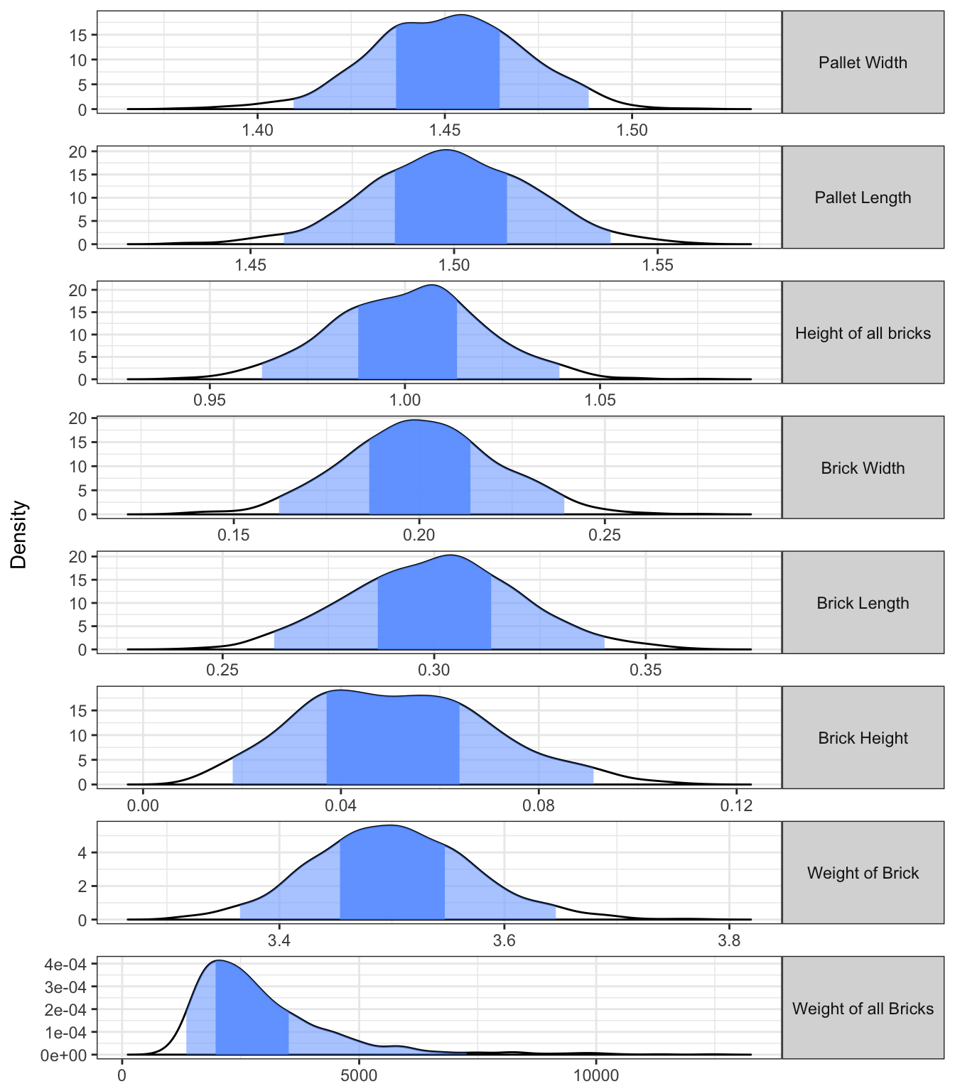
# Compute quantiles (don't just show them)
(quants <- quantile(d$`Weight of all Bricks`, prob=c(0.025, 0.25, 0.75, 0.975)))
## 2.5% 25% 75% 97.5%
## 1345.665 1948.135 3523.359 7281.592# Also compute measurement without uncertainty propogation
(without.prop <- 3.5*(1.45*1.5*1)/(0.2*0.3*0.05))## [1] 2537.5From this figure we can see that we actually have quite a bit of uncertainty in the weight of all the bricks. The light blue region shows the 95% probability region while the 75% region is shown in the darker blue. From this we can see that there is a 75% chance that the total weight of bricks will be between 1950 and 3520 kilograms. However, we also see that our 95% region is huge (1350 to 7280 kilograms) and therefore that we would likely need a more precise measurement device in order to be more certain of the total weight.
On the other hand, if we just ignored the uncertainty propagation (you can imagine someone arguing that they should because the uncertainty in each measured quantity is “small”) then you would simply calculate that the weight of all the bricks is 2537 kilograms. We can see that this number really doesn’t capture the full story.
Improving Back of the Envelope Calculations
Just as a quick point: notice that everything we have done here can be extended to approximate calculation where we guess at values to get an estimate of a calculated quantity. However, if we also estimate the our uncertainty in our guesses we can also get an idea of how uncertain we should be in the calculated quantity.
Lets go through a quick example. Imagine we are trying to estimate the volume of the earth. I’m going to guess that the diameter of the earth is about 10,000 kilometers (I heard someone quote this value once). But I also realize that I am probably off in that guess. How off? I will model my uncertainty about my guess as a normal distribution with a standard deviation of 2500 kilometers (e.g., I think there is about a 68% chance that the true value is between 7,500 and 12,500 kilometers). So whats the volume in liters? To answer this question I am going to assume the earth is a perfect sphere.
t <- 1000
kms <- rnorm(t, mean=10000, sd=2500)  # sample values our guessed distribution
volume.km3 <- (4/3)*pi*(kms/2)^3      # volume in cubic kilometers
liters <- volume.km3*1e12             # convert to liters
data.frame("Diameter of Earth (Kilometers)" = kms,
           "Volume of Earth (Liters)" = liters,
           check.names=FALSE) %>%
  plot_error_quantiles() +
  facet_wrap(~f, ncol=1, scales="free", strip.position="right") +
  theme(axis.title.x = element_blank())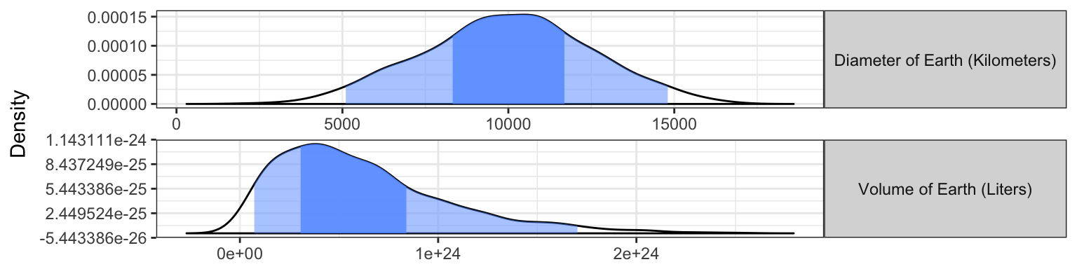
This website lists the earth volume as 1.083e+24 liters. Assuming that website is correct, the true value for the Earth’s value in liters corresponds to the 86-th percentile of our distribution of Volume of the earth. The crucial point here is not that I am correct in my guess. The crucial point is that by estimating the uncertainty in my guess, I was able to somewhat accurately estimate how uncertain I should be in my estimated answer. This can be a very useful tool that I find myself using quite frequent in everyday research and brainstorming.
More Resources
For those interested in learning more of traditional error analysis, beyond what I have discussed in this post, I recommend the book An Introduction to Error Analysis by John Taylor (one of my favorite Authors and one of my favorite cover photos for any textbook).
In addition, for those interested more in simulation studies and quantification of uncertainty I would recommend reading a little bit on Monte Carlo Simulations and Bayesian Statistics.
Code for Plotting
Below I give the code I used to create the plots with shaded quantiles.
print(plot_error_quantiles)## function(d, x.lim=NULL, scales = "free_y"){
## cn <- colnames(d)
## d <- d %>%
## gather(f, dist)
##
##
## d.summary <- d %>%
## group_by(f) %>%
## summarize(p2.5 = quantile(dist, p=0.025),
## p25 = quantile(dist, p=0.25),
## mean = mean(dist),
## p75 = quantile(dist, p=0.75),
## p97.5 = quantile(dist, p=0.975)) %>%
## as.data.frame()
## rownames(d.summary) <- d.summary$f
##
## d.density <- d %>%
## split(.$f) %>%
## map(~with(density(.x$dist), data.frame(x,y))) %>%
## map(as.data.frame) %>%
## bind_rows(.id="f") %>%
## mutate(gt.p25 = x >= d.summary[f,"p25"],
## lt.p75 = x <= d.summary[f,"p75"],
## include.25.75 = gt.p25 & lt.p75,
## gt.p2.5 = x >= d.summary[f,"p2.5"],
## lt.p97.5 = x <= d.summary[f,"p97.5"],
## include.2.5.97.5 = gt.p2.5 & lt.p97.5) %>%
## mutate(f = factor(f, levels = cn))
##
##
## p <- d.density %>%
## ggplot(aes(x = x, y= y))+
## geom_area(fill="white", alpha=0.3, color="black") +
## geom_area(data = subset(d.density, include.2.5.97.5==TRUE), fill="#619CFF", alpha=0.5) +
## geom_area(data = subset(d.density, include.25.75==TRUE), fill="#619CFF", alpha=0.8) +
## facet_grid(f~., scales=scales) +
## theme_bw()+
## theme(strip.text.y = element_text(angle = 0)) +
## ylab("Density")+
## xlab("x")
## if (!is.null(x.lim)) p <- p + xlim(x.lim)
## p
## }