Building the ILR from the ALR Transform
Following up on a recent post on limitations of the ALR and Softmax transforms, I wanted to briefly show how we can derive an Isometric Log-Ratio transform from the Additive Log-Ratio (ALR) transform.
The ILR transform is just an orthonormal basis in the simplex with respect to the Aitchison metric (which follows naturally from using log-ratios - I will probably have a post explaining this more in the future). We are going to use the Gram-Schmidt orthonomalization process to build an orthonormal basis given a set of vectors which are not orthonormal (the coordinates defined by our ALR transform). This is actually the same approach used when the ILR transform was first described. In particular we will use the QR decomposition which is essentially the same as the Gram-Schmidt orthonomalization.
In order to set up the problem in a manner that allows us to use the QR decomposition we will need to rewrite the ALR in matrix form. \[alr(\mathbf{x}) = \mathbf{y} = \left(\ln \frac{x_1}{x_D}, \dots, \ln \frac{x_{D-1}}{x_D}\right)\] This can instead by written as a non-linear log-transform and a linear matrix operation as follows: \[ alr(\mathbf{x}) = \mathbf{y} = \ln(\mathbf{x})\cdot D = \ln(\mathbf{x})\cdot\begin{pmatrix} 1 & 0 & \cdots & 0 \\ 0 & 1 & \cdots & 0 \\ \vdots & \vdots & \ddots & \vdots \\ 0 & 0 & \cdots & 1 \\ -1 & -1 & \cdots & -1 \end{pmatrix}\]
Where we have introduced the matrix \(D\) which represents a linear transformation of the log-transformed data into the log-contrasts defined by our chosen ALR basis (where we have chosen the D-th component as the reference here).
We can create an orthonormal basis by preforming Gram-Schmidt orthonormalization on \(D\); we will call the result \(V\). The ILR transform can now be written as \[ilr_V(\mathbf{x}) = \ln(\mathbf{x})\cdot V\] with inverse transform given by \[ilr_V^{-1}(\mathbf{y}) = \mathcal{C}[exp(\mathbf{y}\cdot V^t)]\] where \(\mathcal{C}(\mathbf{a})= \left( \frac{a_1}{\sum_i a_i}, \dots, \frac{a_D}{\sum_i a_i} \right)\) is the closure operation.
In this form the ILR really looks just like the ALR! We have just done some linear algebra on the matrix \(D\) to turn it into the orthonormal basis defined in \(V\)!
Demonstration
First load packages:
library(compositions) # for plotting ternary diagrams
library(philr) # to compare to results of previous writeup
Now defining D and the Gram-Schmidt orthonormalized version of \(D\) which we will call \(V\).
(D <- rbind(diag(2), -1))## [,1] [,2]
## [1,] 1 0
## [2,] 0 1
## [3,] -1 -1(V <- qr.Q(qr(D))) # The "Contrast Matrix" of the orthogonal basis## [,1] [,2]
## [1,] -0.7071068 0.4082483
## [2,] 0.0000000 -0.8164966
## [3,] 0.7071068 0.4082483Next lets look at the coordinates in the simplex defined by this contrast matrix we created \(V\). That is, lets look at the coordinates of the ILR transform we just created.
coords <- as.matrix(rbind(cbind(0, seq(-1, 1, by=0.1)),
                          cbind(seq(-1, 1, by=0.1), 0)))
plot(ilrInv(coords, V))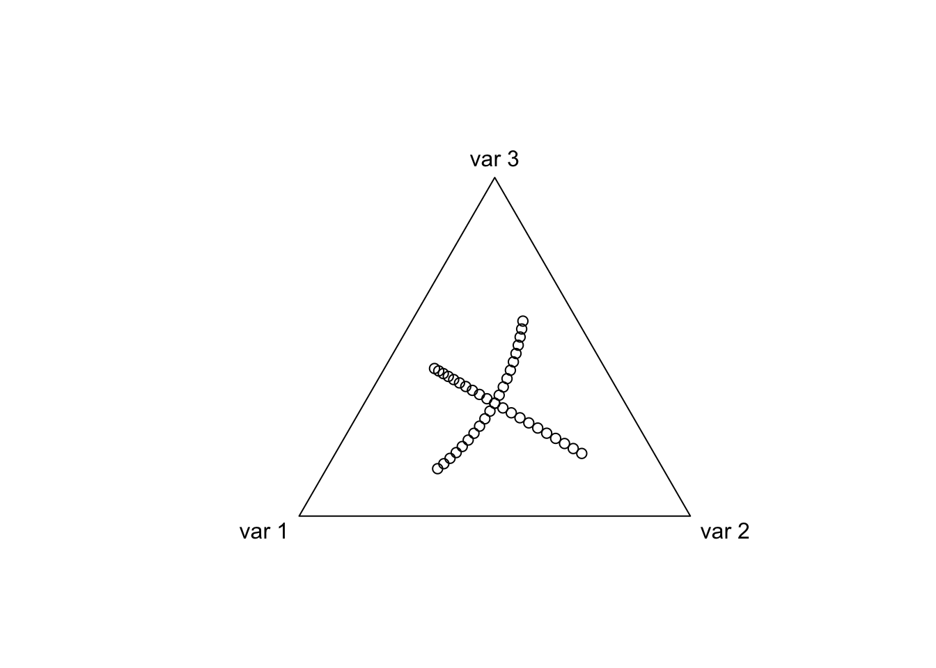
Now to compare to previous write-up, lets create a circle in one basis (which we will define based on a sequential binary partition) and then transform it into the basis we just created. We should see the same circle suggesting that our created basis (while it was not created with a sequential binary partition) is a valid ILR basis.
phy1 <- named_rtree(3)
t <- seq(0, 2*pi, by = 0.1)
x <- cos(t)
y <- sin(t)
circ1 <- cbind(x, y)
colnames(circ1) <- c("n1", "n2")

par(mfrow=c(1,2))
plot(circ1, asp=1)
plot(unclass(ilr(philrInv(circ1, tree = phy1), V = V)), asp=1)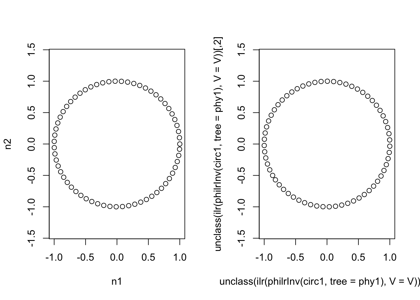
As it turns out, what we ended up creating corresponds to a sequential binary partition but this does not necessarily need to be the case. Think of it like this: there are 3 possible sequential binary partitions of 3 variables but there are an infinite number of rotations of a basis defined by a sequential binary partition. Thus there are an infinite number of ILR transformations for 3 variables (each corresponding to a rotation of the orthonormal basis) but only three of those correspond to sequential binary partitions.