We can do better than the ALR or Softmax Transform
In multiple places in the Compositional Data Analysis literature (for example here and here) people refer to the Additive Log-Ratio transform (ALR) as “not preserving metric concepts”. But what exactly does this mean and how can we visualize this problem?
Here I am going to briefly describe how this problem can be seen with the ALR transform and then show how the Isometric Log-Ratio (ILR) transform does not have this problem.
Note 1: The ALR transform is just a softmax transform that decreases the dimension of the transformed space by 1. The softmax transform has 1 too many dimensions compared to the dimensions of information in the simplex.
Note 2: I just want to be clear: I often find the ALR transform very useful for data analysis (its not all bad). That said, I do think it is essential to understand its limitations.
The ALR Transform
Assuming we take the D-th component of a composition as reference, the ALR transform is given by \[alr(\mathbf{x}) = \mathbf{y} = \left(\ln \frac{x_1}{x_D}, \dots, \ln \frac{x_{D-1}}{x_D}\right)\]
The inverse operation is given by \[alr^{-1}(\mathbf{y}) = \left( \frac{e^{y_1}}{\sum_ie^{y_i}+1}, \dots, \frac{e^{y_{D-1}}}{\sum_ie^{y_i}+1}, \frac{1}{\sum_ie^{y_i}+1}\right)\]
library(compositions)
library(driver) # can be downloaded from my github (jsilve24/driver)
Now I am going to parameterize a circle in one ALR coordinate system and transform it to another ALR coordinate system, we will see that the circle has been warped.
t <- seq(0, 2*pi, by = 0.1)
x <- cos(t)
y <- sin(t)
circ <- cbind(x, y)

par(mfrow=c(1,2))
plot(circ, asp=1) # Plot the circle in one ALR coordinate system
plot(alr(alrInv(circ, 2),3), asp=1) # Plot in a transormed ALR coordinate system. 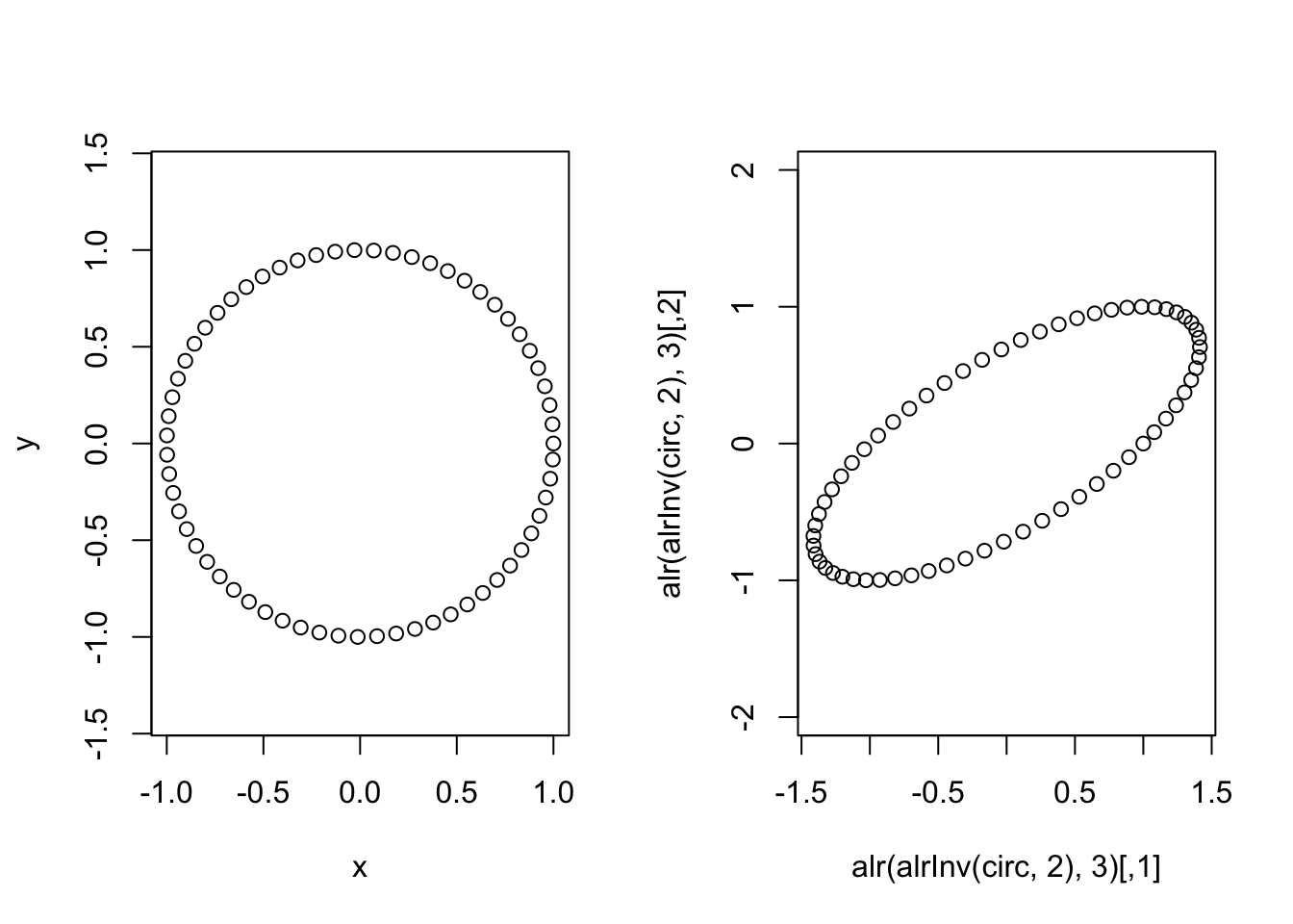
Just to drive the point home, lets look at how distances (as computed by euclidean distances in the transformed space) have changed between these two ALR transforms.
max(dist(circ)) # Max distance between datapoints in original ## [1] 1.999568max(dist(alr(alrInv(circ, 2),3))) # in other alr coordinate system## [1] 3.234656Why does this happen?
The ALR transform corresponds to an oblique coordinate system in the simplex (it is not a basis). More specifically we may say it is oblique with respect to a consistent metric in the simplex (the Aitchison metric).
So lets look at the coordinates induced by the two ALR transforms we just used.
library(compositions)
coords <- as.matrix(rbind(cbind(0, seq(-1, 1, by=0.1)),
                          cbind(seq(-1, 1, by=0.1), 0)))
par(mfrow=c(1,2))
plot(acomp(alrInv(coords, 2))) # One ALR
plot(acomp(alrInv(coords, 3))) # The Other ALR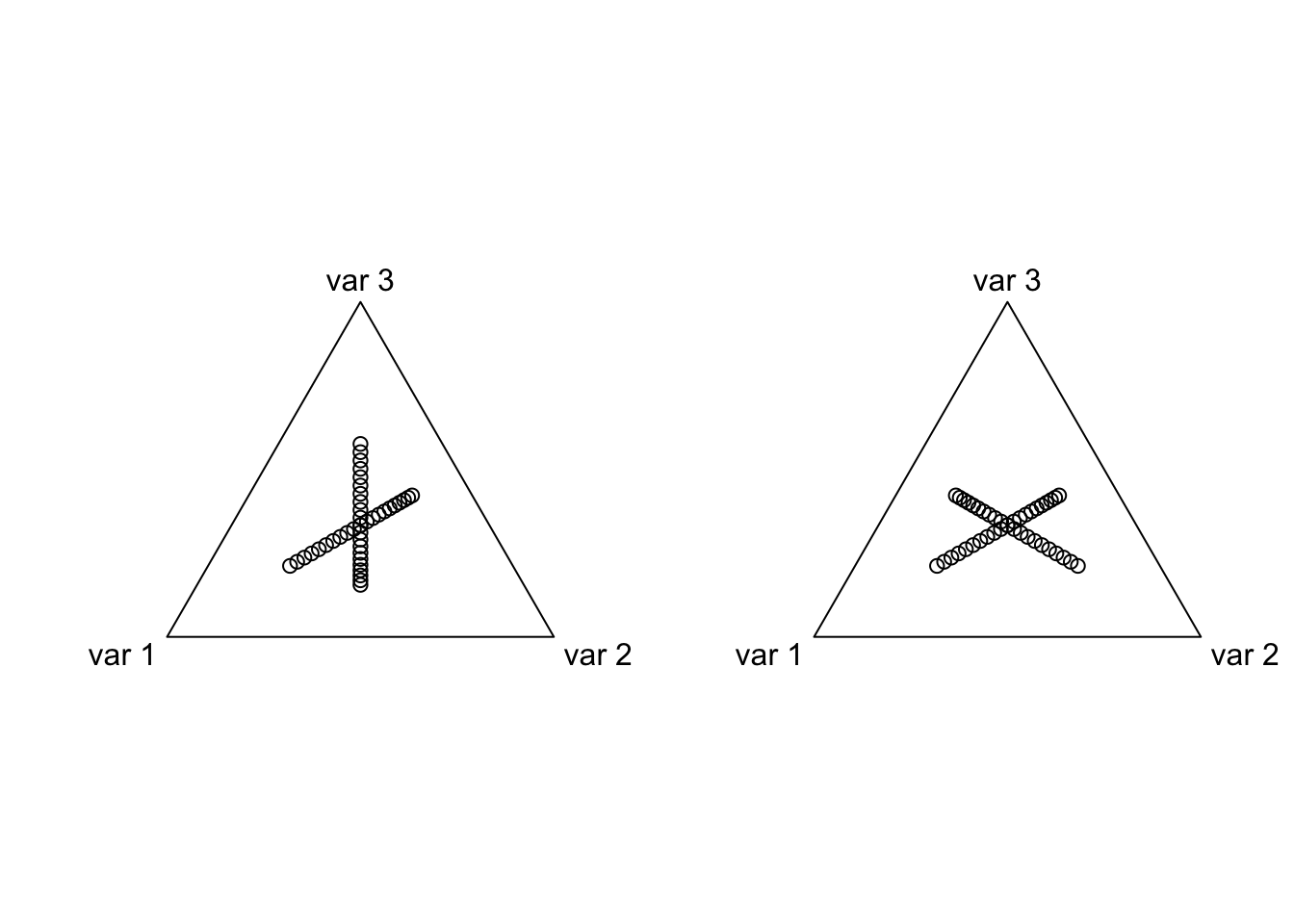
Unfortunately, it can be difficult to build much intuition by looking at these simplex plots. Lets instead look at the coordinates of one ALR transform in terms of the other ALR coordinates
plot(alr(alrInv(coords, 2),3), asp=1) 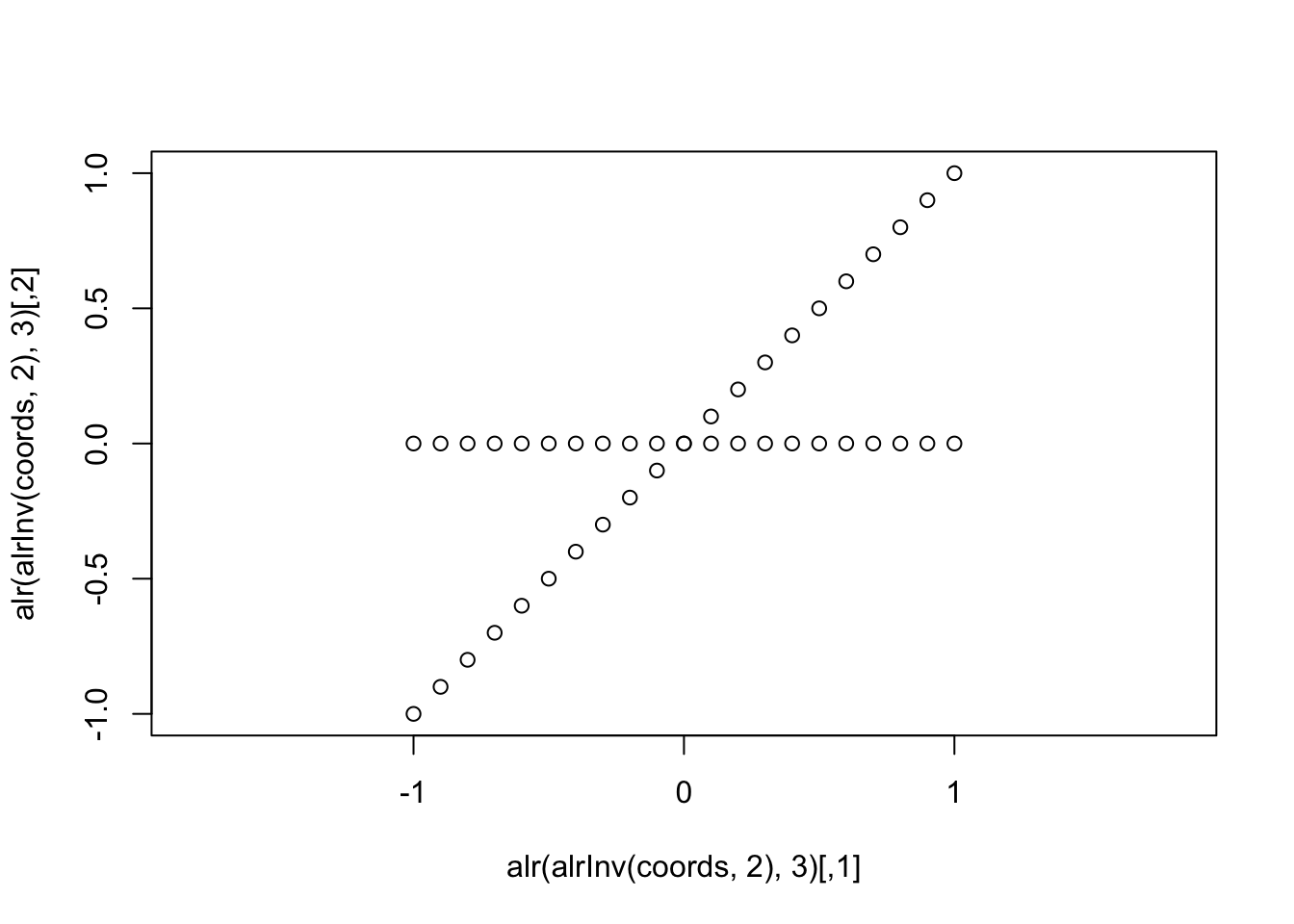
In this form I think it drives home what we mean by “oblique” coordinates, they are not orthogonal (nor do they have unit length so they do not represent an “orthonormal basis”). A careful observer will also notice that the spacing between the points is different for the two coordinates (it is not just a rotation of two lines intersecting at an oblique angle).
This does not happen for ILR/PhILR transforms
While I am not going into much detail about the ILR transform I will just demonstrate that this transform does not have these problems. More details on the ILR transform can be found here. I also use the term PhILR and ILR interchangeably even though the PhILR transform is really just a special case of the ILR transform when the basis is built from a phylogenetic tree. I introduced this name in a recent paper. The crucial point I am trying to make is that we can do better than the ALR/Softmax transform.
library(philr) # Package for building ILR from phylogenetic tree##
## Attaching package: 'philr'## The following object is masked from 'package:driver':
##
## minicloWe can create two different ILR transforms by using two separate sequential binary partitions (we are going to use two random phylogenetic trees).
phy1 <- named_rtree(3)
phy2 <- named_rtree(3)

t <- seq(0, 2*pi, by = 0.1)
x <- cos(t)
y <- sin(t)
circ1 <- cbind(x, y)
colnames(circ1) <- c("n1", "n2")
circ2 <- philr(philrInv(circ1, tree = phy1), tree=phy2)
## Building Sequential Binary Partition from Tree...## Building Contrast Matrix...## Transforming the Data...## Calculating ILR Weights...par(mfrow=c(1,2))
plot(circ1, asp = 1)
plot(circ2, asp = 1)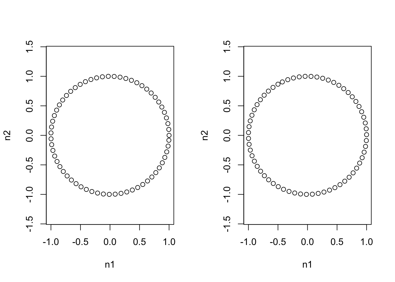
max(dist(circ1)) # Max distance between datapoints in original ## [1] 1.999568max(dist(circ2)) # with respect to other philr transform ## [1] 1.999568Thus we see that in two different ILR bases we get the identical representation of shapes. We also see that distances with respect to the Euclidean metric are respected between different transforms. Now we can look at how this transform looks in the simplex and again when we view one ILR coordinate system in another.
coords <- as.matrix(rbind(cbind(0, seq(-1, 1, by=0.1)),
                          cbind(seq(-1, 1, by=0.1), 0)))
colnames(coords) <- c("n1", "n2")
par(mfrow=c(1,2))
plot(acomp(philrInv(coords, tree=phy1)[,c("t1", "t2", "t3")]))
plot(acomp(philrInv(coords, tree=phy2)[,c("t1", "t2", "t3")]))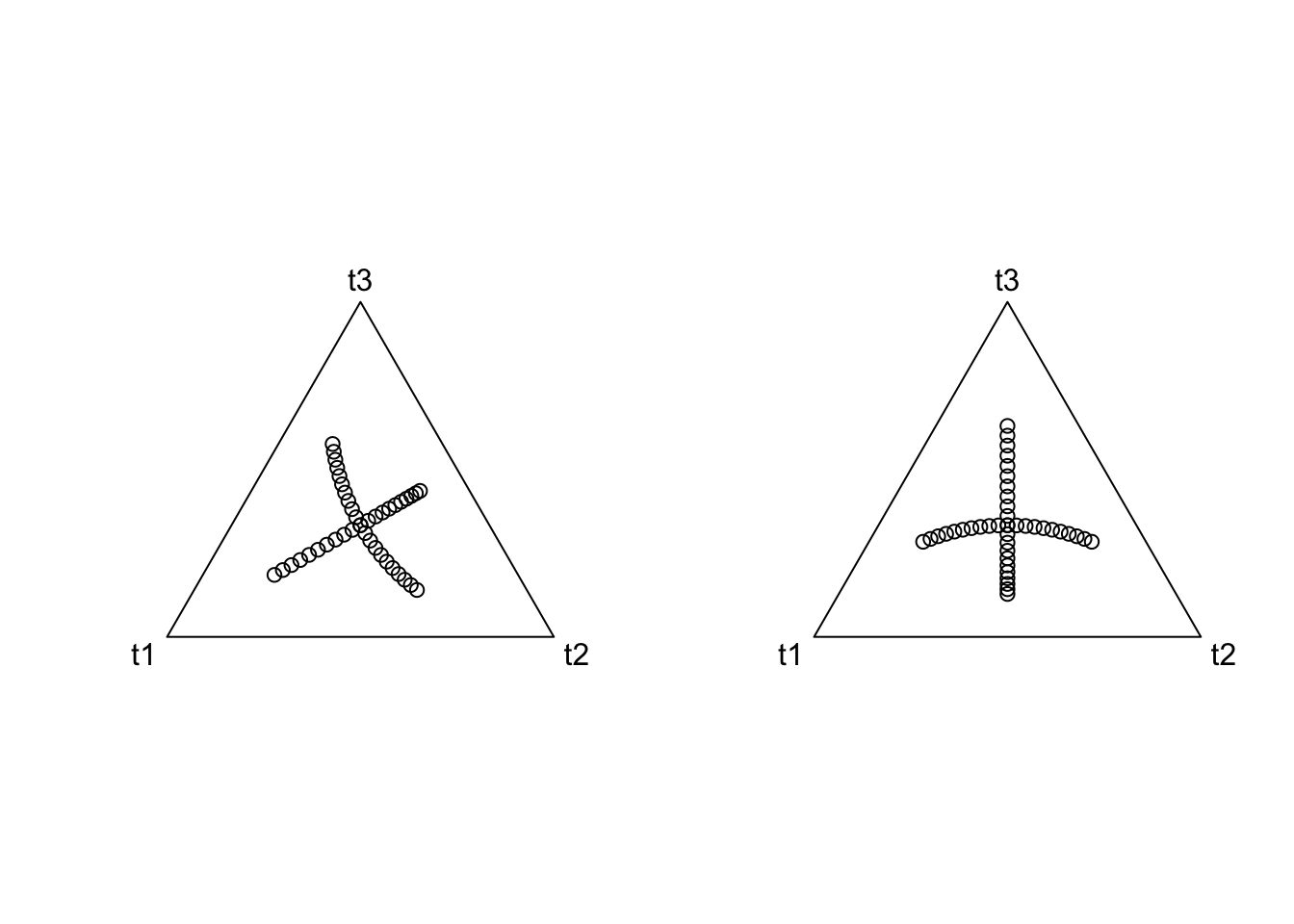
Thus we see that two different ILR bases are just rotations of each other. But what is more important is what one coordinate system looks like with respect to another.
plot(philr(philrInv(coords, tree=phy2), tree=phy1), asp=1)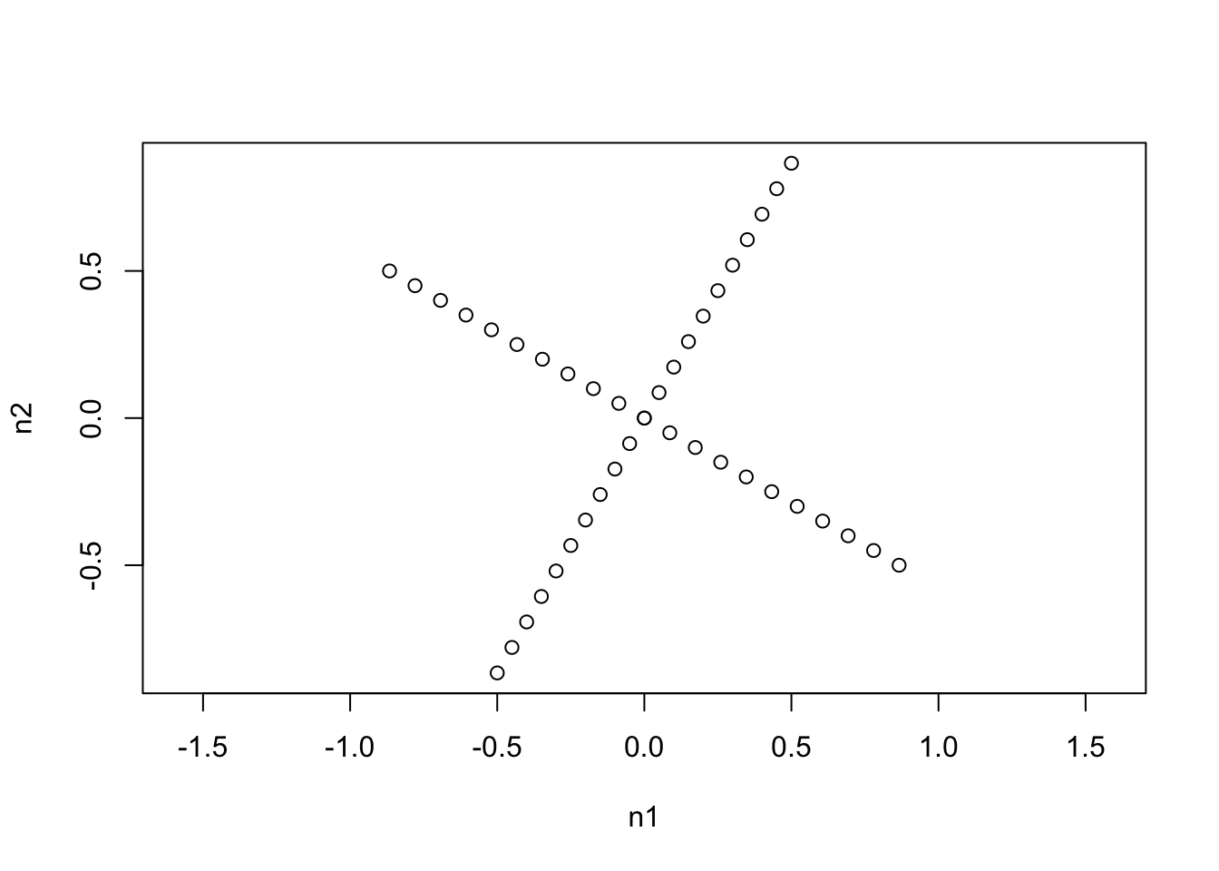
We see that one ILR basis is just a rotation of the other that maintains the orthogonality of the coordinate system. (Actually the ILR transform represents an orthonormal basis in the simplex with respect to the Aitchison metric).
Final Note on Centered Log Ratio (CLR) Transform
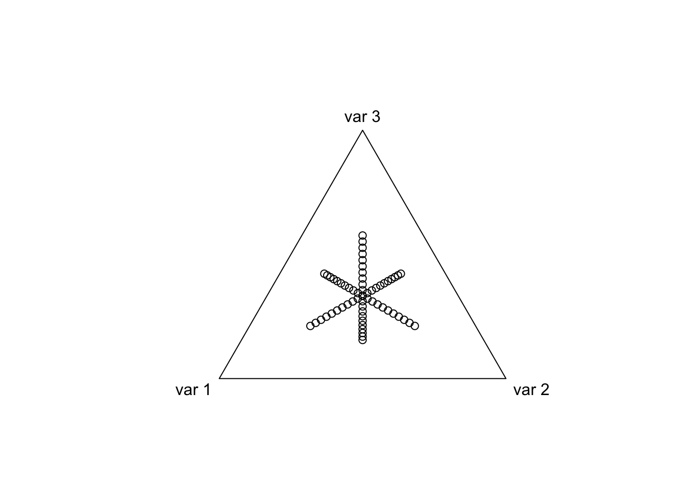
As a final point I just wanted to show what the coordinates of the CLR transform look like in the simplex (to help build intuition for interested readers).
coords <- as.matrix(rbind(cbind(0, 0, seq(-1, 1, by=0.1)),
                          cbind(0, seq(-1, 1, by=0.1), 0),
                          cbind(seq(-1, 1, by=0.1), 0, 0)))
plot(compositions::clrInv(coords))