Visualizing the Multinomial in the Simplex
Lately I have been working on figures for a manuscript. In this process I created a few visualizations that I thought might help others visualize the Multinomial distribution. I will focus on describing how counting processes introduce uncertainty into estimates of relative abundances and I will end with a discussion of how understanding the Multinomial has impacted my view of analyses of sequence count data (e.g., data from 16s studies of the microbiome, RNA-seq, and more). Here I have chosen to focus on the Multinomial distribution, however, much of what I discuss also relates to the Multivariate Hypergeometric Distribution as well.
The Multinomial distribution is a very important distribution that provides a good model for many real world counting processes. Think about drawing \(n\) balls from an urn of infinite size containing \(D\) different colors of balls. Due to our assumption of the infinite size of the urn, we don’t worry about the total number of balls of each color in the urn, we simply work with the relative abundances \(\mathbf{p} = (p_1, \dots, p_D)\) of each color of ball. We describe such relative abundances as elements of a “simplex” (basically just s \(D\) dimensional triangle) such that all elements \(p_i\) are positive and \(\sum_i p_i = 1\).
When dealing with such count data, it is often of interest to estimate the proportions/relative abundances in the population being sampled. Let a random draw of \(n\) balls be denoted by the vector of counts \((x_1, \dots, x_D)\) in which the element \(x_i\) denotes the number of balls of color \(i\) drawn. The maximum likelihood estimates for the proportions of each color ball in the urn (i.e., the ML estimates for the Multinomial parameters) are given by \[\hat{\mathbf{p}} = \left(\frac{x_1}{\sum_ix_i}, \dots, \frac{x_D}{\sum_ix_i}\right).\] In other words, the maximum likelihood estimates are simply the relative abundance of each type of ball in our sample. Below I provide a function for visualizing the Multinomial distribution in terms of these maximum likelihood estimates \(\hat{\mathbf{p}}\).
A Function To Aid in Plotting
First I am going to write a function to help visualize the Multinomial in terms of its parameter support.
library(tidyverse)
library(driver) # https://github.com/jsilve24/driver
library(combinat)
library(ggtern)

# Function to help plotting
# n - number of samples
# p - vector of probabilities (length = 3)
plot_ternary_multinomial_density <- function(n, prob){
  sx = t(xsimplex(p=3,n=n))
  dx = apply(sx, 1, function(x) dmultinom(x, size=n, prob=prob))
  sx <- cbind(as.data.frame(miniclo(sx)), dx)
  colnames(sx) <- c("v1", "v2", "v3", "d")

  s <- ggtern(sx, aes(x=v1, y=v2, z=v3)) +
    geom_point(alpha=0.4, aes(size=d/max(d))) +
    theme_bw() +
    guides(size=FALSE) +
    scale_size(range=c(.1, 2))
  s
}
Building Some Intuition for the Multinomial Distribution
Next I am going to point out a few features of the Multinomial distribution. I will depict the three types of things we are counting (they could be different colors of balls) as v1, v2, and v3.
A Discritization of the Simplex
The Multinomial has a continuous parameter space, that is the vector \(p\) contains elements that are continuous and not discrete. However, Multinomial counting processes results in a discretization continuous parameter space.
prob <- miniclo(c(.37, .37, .3))
d <- setNames(as.data.frame(prob), c("v1", "v2", "v3"))
plot_ternary_multinomial_density(10, prob) +
  geom_point(data=d, color="red", size=2, fill="red")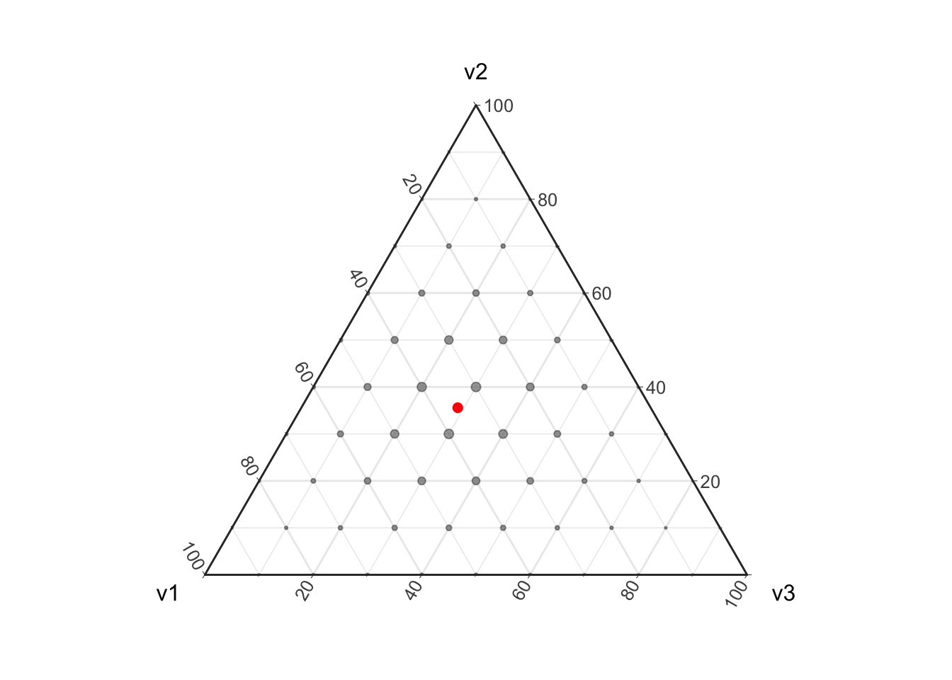
Given a finite sample (e.g., non-infinite \(n\)) we can only obtain a finite set of possible parameter values. If this does not make sense yet think about flipping a coin twice, there are 4 possible outcomes \(\{(H,H), (H, T), (T, H), (T, T)\}\) leading to 3 possible estimates for the underlying proportions \(\{(1, 0), (.5, .5), (0, 1)\}\). In this coin flipping example we cannot get a maximum likelihood estimate of \((0.3, 0.7)\). In the above visualization I have highlighted the true proportion that this Multinomial distribution is based on in red; note that with a sample of size 10 there is no way to perfectly estimate this “true” proportion. This discretization of the proportions is important to take into account when estimating proportions from count data as it introduces uncertainty into the resulting estimates.
Effect of changing \(n\) (counting as a random process)
Uncertainty in the Multinomial parameters is not simply due to the discretization of the parameter space. Uncertainty in these estimates also arises because we are modeling counting as a random process. Note that as we draw more and more balls out of the urn the Multinomial distribution concentrates around the true value. This is because drawing more balls is like having more replicates in an experiment, eventually (in the absence of bias) our estimates will start concentrating around the true value.
d <- setNames(as.data.frame(prob), c("v1", "v2", "v3"))
plot_ternary_multinomial_density(100, prob) +
  geom_point(data=d, color="red", size=2, fill="red")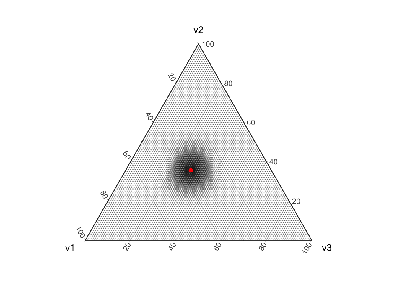
Effect of changing \(\mathbf{p}\) (focus on boundaries)
Based on the above figures, it may seem simple to estimate proportions from count data, just collect at least 100 or so counts and you have a pretty good covering over the simplex. But this is often not the case in real world problems! In reality we are often confronted with situations in which some of the relative abundances are very small compared to some others (e.g., one color of balls is much more rare than another color). In addition, the difference between a zero proportion and a non-zero but small proportion is often very important (think about the difference between estimating that one type of ball is completely absent from an urn versus estimating that it is present but at much lower proportion than the other types of balls). In this situation it can become quite difficult to obtain enough samples to accurately estimate a non-zero proportion for the rare type of ball.
prob <- miniclo(c(.9, .091, .005))
p1 <- plot_ternary_multinomial_density(100, prob) +
  geom_point(data=setNames(as.data.frame(prob), c("v1", "v2", "v3")), color="red", size=2, fill="red")

# Lets also zoom in on this region
p2 <- p1 + theme_zoom_L(0.2)

# Now put these two plots side-by-side
grid.arrange(p1, p2, ncol=2)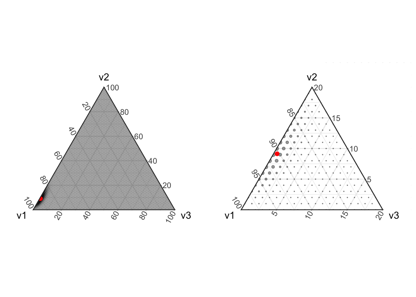
In the above figure we see that with only 100 counts, the majority of the distribution centers on estimating the component v3 with a relative abundance of zero even though the true simulated value is small but non-zero.
Implications for Real World Data
I would like to point out that this behavior of the Multinomial distribution results from a “statistical competition to be counted” between the components. We are only sampling \(n\) balls total, therefore having more of one type of ball will result in us measuring fewer counts from other types of balls. This does not mean that there is actually any interaction between the balls, simply that the way we are measuring the composition of the urn induces a correlation between the types of balls.
I have been seeing a lot of papers recently that seem to ignore this feature of their data generation process. For example, with next-generation sequencing technologies a large amount of DNA processed and only a small amount of that DNA is ever actually counted during sequencing. As a result of this there is the same type of “competition to be counted”, more of one type of DNA transcript will lead to fewer counts from other transcripts. Despite this, many analyses ignore this and draw inferences regarding the behavior of individual transcripts (e.g., differential abundance analyses). Also please note that I would welcome comments from readers who disagree with my opinion!
That said, simply transforming counts to relative abundances by dividing the counts by the total (e.g., the Maximum Likelihood estimate for the Multinomial) as is commonly done with sequence count data does not make much sense to me either. The counting process does not allow us to measure relative abundances directly. As I pointed out above, the discretization of the underlying simplex and the uncertainty introduced by the random nature of counting are also essential components to account for, especially in the presence of very uneven relative abundances (e.g., when some transcripts/balls are very low abundance compared to others).