Measure Theory Made Ridiculously Simple
During my first few years of medical school I became a big fan of the [Subject] Made Rediculously Simple book series (as in Clinical Microbiology Made Rediculously Simple). I found that the authors did a great job of simplifying the subject matter, sometimes to the point of absurdity, while getting the core concepts across in a memorable way. For some time now I have wished that similar tools were available for mathematics. While I may not have the same artistry or comical flare that those authors have, here I attempt to take the Made Rediculously Simple flare to explain some of the core concepts of measure theory. This post is designed for those who have a background in basic calculus and recognize that measure theory plays some important (although perhaps cryptic) role in modern probability and statistics.
I have heard a number of people say that they have a hard time understanding measure theory. I think the confusion is very understandable, the discussion of measures are often complicated by the need to introduce the formalism of \(\sigma\)-algebras and the Borel \(\sigma\)-field and thus students can often feel overwhelmed by the sheer number of new abstract definitions and concepts that must be understood all together. I am very thankful that I have had some really good mentors who have distilled the concepts of measure theory to a point that seems very intuitive to me. In this post I will try to convey a very rough but intuitive introduction to measure theory in the hopes that it may serve as a less confusing gateway to the subject. Please note that I have sacrificed some mathematical rigor and correctness in my attempt to divorce the concepts of measures from set theory. Instead I try to convey an intuitive notion of some concepts in measure theory and then explain why the set theory definitions are needed at the end.
Why should I care?
The first question I wanted to just briefly touch on is: Why should I care about measure theory?
The Theoretical Answer
The theoretical answer is that measure theory literally underlies the entire notion of random-variables, probability, and statistics. In fact, studying measure theory has helped me conceptualize the question: Why should I bother using the concept of probability at all?
The Applied Answer
That said, I realize this theoretical answer may not appeal to the more applied person who will want to know how these concepts can be used in statistical practice. To such a person I would admit that (currently) the applications of measure theory in statistics seems largely relegated to researchers studying new types of data and doing methodological research; however, there is a growing number of tools that actually use measure theory concepts directly in the analysis of real-world data sets. For example, in the field of compositional data analysis, changing the reference measure of the simplex has turned out to be a powerful method to up or down-weight certain variables in an analysis (Egozcue and Pawlowsky-Glahn 2016). Another cool example is the use of measure theory in the study of Bayes Linear spaces which give a vector space structure to the space of probability densities (van den Boogaart, Egozcue, and Pawlowsky-Glahn 2014).
As a final note, I would point out that re-expressing a density with regards to a different reference measure can make working with some fairly intractable densities possible. For example, the Logistic-Normal distribution is a fairly difficult distribution to work with directly (e.g., its mean and variance have no analytical closed form with respect to the Lebesgue measure). However, reparameterization of this distribution in terms of log-ratios converts this nasty distribution into the multivariate normal distribution. In Mateu-Figueras, Pawlowsky-Glahn, and Egozcue (2013), the authors show that this reparameterization is actually equivalent to changing the reference measure from the standard Lebesgue Measure to the Aitchison Measure. In essence, they show that changing the reference measure can make a seemingly intractable density tractable.
The meat of this post (start here if short on time)
I would say that many concepts in measure theory can be seen as a generalization of the following image:
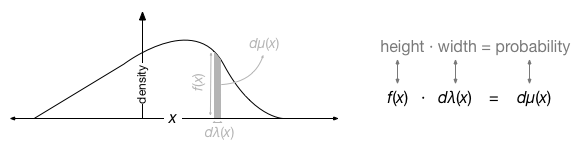
Essentially a probability measure is a generalization of a volume element. \(\mu(x)\) is a probability measure, essentially a function that takes in an interval or a set of points and outputs a positive real value representing the “area/volume” (or amount) of probability in the specified region. As a point of terminology, we refer to \(\mu(x)\) as the probability measure, \(\lambda(x)\) as the reference measure, and \(f(x)\) as the probability density function. Note that we often take \(\lambda(x)\) as the Lebesgue Measure which is essentially just a uniform function over the sample space (i.e., the Lebesgue measure is what you would probably think to do by default before you even learned about measure theory).
The probability measure \(\mu(x)\) is really the crucial probabilistic object we use for modeling. It is the probability measure that tells us the probability of an event \(x\). The reference measure \(\lambda(x)\) is essentially just a meter-stick that allows us to express the probability measure as a simple function \(f(x)\). That is, we represent the probability measure \(\mu(x)\) as \(f(x)\) by comparing the probability measure to some specified reference measure \(\lambda(x)\). This is essentially the intuition that is given by the Radon-Nikodym derivative \[f(x) = \frac{d\mu(x)}{d\lambda(x)}\] or equivalently (height = area/width). Note that we can also represent the same idea by \[\mu(A) = \int_{A\in X}f(x)d\lambda(x)\] where \(\mu(A)\) is the sum of the probability of events in the set \(A\) which is itself a subset of the entire sample space \(X\). Note that when \(A=X\) then the integral must equal 1 by definition of probability.
Reexpressing a density with respect to a different reference measure
Just to point out how much basic calculus and algebra can extend our intuition for measure theory, I will briefly discuss how you can re-express a given density \(f(x)\) with respect to a different reference measure. Changing the reference measure is kind of like stretching or squishing the density around on the \(x\) axis. As you stretch or squish the density you keep the total volume constant even though the height of the density \(f(x)\) changes. That is, by changing the reference measure (stretching or squishing) you can change the functional form of the density \(f(x)\) while keeping the core concept (the association of probability to events, which is given by the probability measure \(\mu(x)\)) the same. Note also the Radon-Nikodym Chain Rule shows us how to re-express a density with respect to a different measure (note this is essentially basic calculus and algebra). Lets say you want to re-express the density of \(f(x)\) with respect to a compatible measure \(\omega(x)\), then we have \[ f_\omega(x) = \frac{d\mu(x)}{d\lambda(x)}\frac{d\lambda(x)}{d\omega(x)} = \frac{d\mu(x)}{d\omega(x)}. \] Thus while \(f(x)\) may be very difficult to work with, it is possible that \(f_\omega(x)\) (which represents the same probabilistic object) is much easier to work with (think the Logistic Normal and the link to the Multivariate Normal as I mentioned briefly above).
So why all the set theory?
Hopefully this description of measure theory is much more approachable than those that start by defining \(\sigma\)-algebras and the Borel \(\sigma\)-field. However, the question must be broached, why then the need for this complicated set theory? Here I have made use of our familiarity with Real space to try to get the core concepts of measure theory across, but measure theory is much more powerful and general than just measures of probability over Real space. For example, imagine defining a probability distribution over permutations of objects. You can imagine that the definition of area/volume and width, are likely going to need to need to be generalized to this much less intuitive space of permutations. Essentially the language of \(\sigma\)-algebras/fields gives the necessary formalism to generalize these definitions. The Borel \(\sigma\)-field is simply a special definition for \(\sigma\)-fields over open intervals in Real space. We need this formalism because it can be difficult to work with the infiniteness of Real space.
More Resources to Learn From
For those that want to learn more about measure theory, I would recommend starting with the excellent 4 page tutorial A Measure Theory Tutorial (Measure Theory for Dummies) by Maya R. Gupta. This tutorial is a nice bridge between the almost reckless disregard for formality I present and the crucial definitions and terminology that are the foundations of measure theory. I encourage readers to pay particular attention to the section entitled “The truth about Random Variables”. At the end of this tutorial she gives a number of recommendations for introductory texts on the subject.
One Final Point (Warning: Abstractitude Sickness or The Flatlander’s Glimpse Ahead!)
Just as another cool connection to draw, note the very close (but not exact) relation between differential forms and measures and the connection between differential forms, changes of measures (e.g., the chain rule for the Radon-Nikodym derivative), and the transformation of variables formula that is taught in first year statistics courses!
To spark some ideas: \[ g(y) = f(x)\left\vert\frac{dx}{dy} \right\vert \] which implies that \(g(y) \vert dy\vert = f(x) \vert dx \vert = d\mu(x)\). I believe that here \(\vert dx\vert\) and \(\vert dy \vert\) can be taken as the Lebesgue measures for the sample spaces \(X\) and \(Y\) respectively (\(d\lambda(x)\) and \(d\lambda(y)\)). From the above discussion we could also write \[ g(y) = \frac{d\mu(x)}{d\lambda(x)}\frac{d\lambda(x)}{d\lambda(y)}\] which is essentially identical to what the chain rule for the Radon-Nikodym derivative.
References
Egozcue, J. J., and V. Pawlowsky-Glahn. 2016. “Changing the Reference Measure in the Simlex and Its Weightings Effects.” Journal Article. Austrian Journal of Statistics 45 (4): 25–44.
Mateu-Figueras, G., V. Pawlowsky-Glahn, and J. J. Egozcue. 2013. “The Normal Distribution in Some Constrained Sample Spaces.” Journal Article. SORT 37 (1): 29–56.
van den Boogaart, K. V., J. J. Egozcue, and V. Pawlowsky-Glahn. 2014. “Bayes Hilbert Spaces.” Journal Article. Australian and New Zealand Journal of Statistics 56 (2): 171–94.